Amy Gainer
Statistical Analysis
1) Data Checking
At each depth interval, each treatment was checked for outliers, normality and equal variances. Boxplots were initially used as a visual check for outliers and normality(G-1, G-2). Residuals of treatments at each depth were determined. Histograms of the residuals were used as a normality check but due to small sample size was not a good representation of real distribution (A-3). Residuals were used for normality testing rather than checking each treatment individually without using residuals because the former is less time consuming. Residuals were calculated for each depth and then a Shapiro test was performed to identify significant departures from normality (Hamman 2009). A Shapiro test p value of greater than alpha (0.05) indicates that the data is more normal. A p value less than 0.05 indicates a small chance that the data is normal. A alpha value of 0.05 is sufficient for this data interpretation because it is not a life or death.
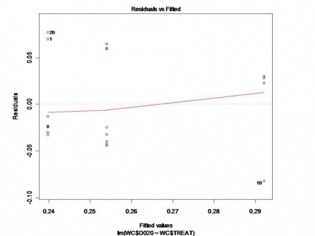
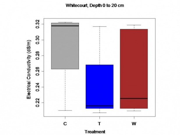
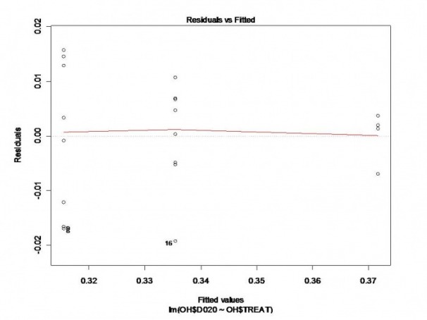
All the data is normally distributed with one exception. At the Whitecourt site, at a depth of 0 to 20 cm, the data is not normally distributed. The Shapiro test confirmed this with a low p value (0.0353) for that particular depth. From the residual plot for this depth, non normality is observed due to unequal distribution of data points around the center line (G-3). By looking at the boxplot of treatments for this depth we can determine that the tap water treatment is the cause of the non normality (G-4). A histogram of the residuals for this depth shows that the shape is similar to the other depths, relatively bell shaped.
From the plot of residuals for each depth, it was observed that the data set does not have equal variance (G-5). This was observed due to the variations in distance from the middle of the plot. The Bartlett`s test was not necessary because unequal variances was obvious from the residual plots.
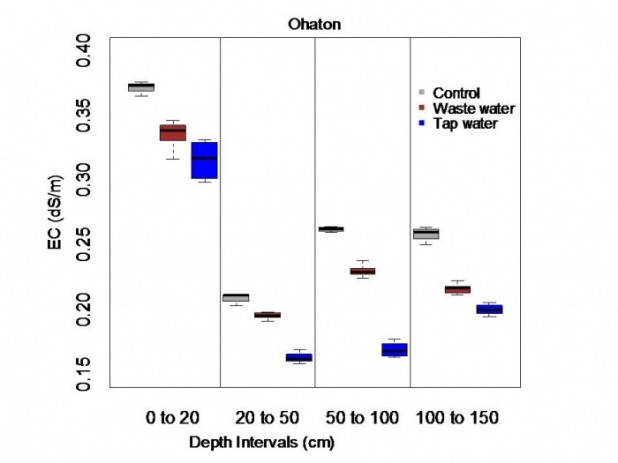
S-1. Boxplot of treatment electrical conductivity (dS/m) at different depth for Ohaton.
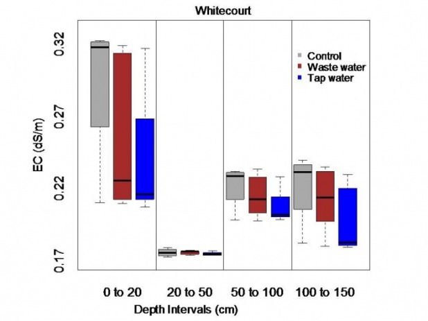
S-2. Boxplot of treatment electrical conductivity (dS/m) at different depth for Whitecourt.
S-3. Plot of residuals for Whitecourt at depth 0 to 20cm.There are not equal
S-4. Boxplot of treatments at Depth 0 to 20 cm showing non normality in Tapwater (T) treatment.
S-5. Plot of residuals for Ohaton for depth 0 to 20 cm. From this you can see that there is normality because the are equal data points on each side of the center line but they are not spaced evenly apart indicating unequal variances.
2)Treatment
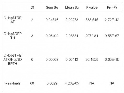
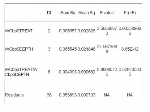
A multi factor ANOVA was performed for each site although there was not equal variances. From the ANOVA (S-6, S-7), both sites had significant differences between treatments. It should be noted that the p value for Whitecourt was 0.03, which is slightly less than 0.05. Due to the this lower significance and unequal variances of data, the effect at this site is still undetermined.
At each depths, t tests were performed between the treatments (A-1). For each depth at each location there was 3 possible combinations, Control(C) vs. Tap water(T), C vs Waste water (W), and W vs T. For Whitecourt site at the depth of 0 to 20 cm where T was found to be non normal. The Wilcoxon test was used when comparing T with C and W. The Wilcoxon test is a t test alternative for non normal data with similar distributions. The null hypothesis for this test is that the true location shift is equal to 0. A p value greater than alpha of 0.05 would indicate that this is true and the treatments are not significantly different. A p value less than 0.05 implies that the null hypothesis is false and that the treatments are significantly different.
For comparing treatments a non parametric test was also performed. A Kolmogorov Smirnoff test was performed when the data was wrongly assumed to be normal and different shaped. The p values from this test were adjusted using Holms adjustment for multiple inferences. The p values derived using this method had higher p values, or less significant differences (A-6). This is because this test is less powerful (Hamman, 2009)
S-6. Multi factor ANOVA table for Ohaton.
S-7. Multi factor ANOVA table for Whitecourt.
3) Depths
From the multi factor ANOVA test, there is significant depth effects at both Whitecourt and Ohaton (S-6, S-7). Differences between treatments at each depth was further investigated using t tests (A-2). Each treatment was compared with the other treatment but at a different depth. For example, there are 6 the possible combinations for comparing Controls between depths: 0 to 20 vs 20 to 50, 0 to 20 vs 50 to 100, 0 to 20 vs 100 150, 20 to 50 vs 50 to 100, 20 to 50 vs 100 150 and 50 to 100 vs 100 to 150. The Wilcoxon test was used when comparing the tap water treatments due to the fact that tapwater at depth 0 to 20 cm is not normal but all depths had similar data shapes. As mentioned above, when the p value is less than the alpha value of 0.05, the depths are significantly different.
.
.
